Introduction
Nontyphoidal
Salmonella (NTS) is a leading cause of diarrheal disease worldwide and contributes substantially to foodborne morbidity and mortality. It is estimated to cause approximately 94 million cases and more than 150,000 deaths annually, although reported estimates vary widely across regions because of differences in surveillance systems and diagnostic capacity [
1]. Although incidence rates are lower than those in sub-Saharan Africa, NTS remains an important public health problem in South and Southeast Asia, where regional estimates suggest a measurable burden. Local studies in Malaysia have documented clinically significant disease, including invasive infections among young children and recurrent foodborne outbreaks in schools and community settings, as well as possible ongoing transmission involving asymptomatic food-handler carriers [
2,
3].
In Malaysia, laboratory-confirmed NTS cases are routinely captured through passive national laboratory surveillance systems, and outbreak investigations are conducted in response to reported food poisoning events. Although NTS infections often show seasonal variation influenced by environmental, climatic, and population-related factors, their temporal dynamics in Malaysia have not been systematically characterized. National laboratory surveillance data can be used to examine these patterns and support more informed, proactive surveillance. Time-series analysis is useful for characterizing long-term trends, seasonality, and short-term fluctuations in infectious disease data; these analyses can also support short-term forecasting and provide a baseline for identifying unusual increases. Autoregressive integrated moving-average (ARIMA) models have been widely used in epidemiology because they are interpretable and can model linear temporal dependencies and seasonality. Seasonal components can also be incorporated to flexibly model the smooth, recurring seasonal patterns commonly observed in foodborne diseases. Recent advances in machine learning, particularly long short-term memory (LSTM) neural networks, may improve modeling of nonlinear dynamics and complex residual structures that conventional statistical models may not fully capture. Hybrid frameworks combine statistical and deep learning methods to model linear and nonlinear dynamics separately [
4], and related approaches, such as ARIMA–support vector machine models, have shown improved forecasting performance in pandemic surveillance [
5,
6]. In addition, the coronavirus disease 2019 (COVID-19) pandemic may have temporarily disrupted disease transmission and surveillance, potentially affecting the validity of time-series forecasts based on historical data [
7]. National-level aggregation may also obscure important regional heterogeneity in disease patterns, with implications for the generalizability of forecasting models and their potential use in surveillance.
This study aimed to characterize the temporal dynamics of laboratory-confirmed human NTS cases in Malaysia between 2018 and 2024, evaluate the performance of time-series models for short-term prediction, assess the impact of the COVID-19 pandemic on the structural stability of the time series, and explore the potential role of model-based approaches in supporting surveillance.
Materials and Methods
Data Source
Malaysia’s national laboratory-based surveillance system requires all
Salmonella spp. isolates from specimens collected in public and private healthcare facilities to be referred to the National Public Health Laboratory (NPHL) and the Ipoh Regional Public Health Laboratory for serotyping and line listing. The Institute for Medical Research coordinates the National Surveillance of Antibiotic Resistance [
8,
9], and outbreak investigations are coordinated through the Public Health Emergency Operations Centre. Since 2018, these workflows have been standardized, ensuring consistent surveillance procedures throughout the study period. The surveillance database includes laboratory-confirmed
Salmonella isolates reported through this centralized referral system, which supports nationwide capture of laboratory-confirmed NTS cases, although case detection may be influenced by healthcare-seeking behavior and testing practices. A laboratory-confirmed NTS case was defined as isolation of a nontyphoidal
Salmonella enterica serovar from any clinical specimen. Nonhuman isolates,
Salmonella Typhi,
Salmonella Paratyphi A,
Salmonella Paratyphi C, and tartrate-negative
Salmonella Paratyphi B were excluded. Deduplication was performed using the database line listing: isolates from the same individual with the same serovar collected within 30 days of the initial specimen were excluded, whereas isolates collected after 30 days or with a different serovar were considered new infection episodes and retained. The study period extended from January 1, 2018, to December 31, 2024, and data were aggregated into monthly case counts according to the laboratory reporting date. For regional assessment, cases were stratified into 6 geographic regions: Central (Kuala Lumpur, Putrajaya, and Selangor), Northern (Kedah, Penang, Perak, and Perlis), Southern (Johor, Melaka, and Negeri Sembilan), East Coast (Kelantan, Terengganu, and Pahang), Sabah, and Sarawak.
Statistical Analyses
Statistical analyses were performed using R ver. 4.4.3 (The R Foundation for Statistical Computing) in the RStudio (PBC) integrated development environment, primarily with the fable, fpp3, and tseries packages [
10–
12]. Hybrid modeling that incorporated LSTM networks was conducted using the
Keras package interfaced through reticulate to integrate the R and Python (Python Software Foundation) environments [
13].
Decomposition analysis and model specification
Seasonal patterns, including intra-annual variation and year-specific monthly effects, were examined using year-stratified seasonal plots and seasonal subseries plots. Seasonal–trend decomposition using Loess (STL) was applied to the monthly NTS time series for 2018–2024 to decompose observed counts into trend, seasonal, and remainder components; a finite seasonal smoothing window of 13 months was used rather than a periodic seasonal specification [
14]. Stationarity was evaluated using the Kwiatkowski-Phillips-Schmidt-Shin (KPSS) test and the augmented Dickey-Fuller (ADF) test, applied to both the original and differenced series [
14]. Autocorrelation function (ACF) and partial autocorrelation function (PACF) plots of the first-order differenced series were examined up to lag 36 to identify appropriate nonseasonal and seasonal autoregressive (AR) and moving-average (MA) terms. The Box-Jenkins framework was used to provide transparent diagnostic assessment while preserving epidemiological interpretability. Order selection was guided by patterns of notable spikes and decay behavior and was validated against an automatically selected specification based on the Hyndman-Khandakar algorithm [
14]. On the basis of the lag structure and the theoretical plausibility of foodborne disease reporting dynamics, competing nonseasonal models, including ARIMA(0,1,1), ARIMA(1,1,0), and ARIMA(1,1,1), were evaluated. Seasonal ARIMA (SARIMA) extensions were also evaluated; however, because strong seasonal autocorrelation was not observed, deterministic seasonal components using Fourier terms were incorporated [
14]. Higher-order Fourier terms (
K=1–3) were tested, where
K represents the number of sine–cosine harmonic pairs used to approximate the annual cycle (m=12 for monthly data). Residual diagnostics were evaluated using ACF plots and the Ljung-Box test. The forecasting performance of the selected ARIMA model was compared with that of standard benchmark models: naïve (NAIVE), seasonal naïve (SNAIVE), random walk with drift (DRIFT), and the mean model [
14]. Exponential smoothing state-space (ETS) models were also fitted using additive error terms, including simple exponential smoothing (SES; level only), Holt’s linear trend model (level and trend), and additive Holt-Winters models (level, trend, and additive seasonality) [
14]. Candidate models were compared using in-sample model adequacy for 2018–2023, including corrected Akaike information criterion (AICc) and residual diagnostics, together with out-of-sample forecasting performance in the 2024 holdout period to identify the most appropriate forecasting model.
Structural stability assessment
Structural stability was assessed to determine whether parameter respecification or restricted training periods were needed. Multiple interrupted time-series (ITS) models were constructed using March 2020 as the intervention point, corresponding to the implementation of nationwide movement restrictions. Three intervention specifications were evaluated: (1) a level-change model estimating an immediate step change from March 2020 onward; (2) a level-and-slope-change model estimating both an immediate level change and a sustained post-intervention trend change from March 2020 onward; and (3) a temporary pulse model, in which the intervention indicator was coded only during the COVID-19 disruption period (March 2020–December 2021) to represent a transient disruption [
15]. All models were specified within the final ARIMA–Fourier framework. The intervention variables used in the ITS analysis were evaluated only to assess structural stability and were not incorporated into the final forecasting model.
Exploratory hybrid ARIMA–LSTM modeling
A hybrid ARIMA–LSTM modeling approach was explored to assess whether modeling the residual series could improve predictive performance. Residuals from the selected ARIMA–Fourier model were extracted, standardized, and structured into 12-month lagged sequences to capture temporal dependencies. Because the sample size was limited, a simple LSTM architecture with a single hidden layer and a dense output layer was specified. To reduce overfitting, early stopping based on validation loss was applied, and a parsimonious set of hyperparameters was selected. The model was trained using the Adam optimizer, with mean squared error as the loss function. Residual forecasts were generated recursively and combined with ARIMA–Fourier forecasts to produce a hybrid forecast as follows: y^t=y^tARIMA+e^tLSTM, where y^tARIMA denotes the linear forecast from the ARIMA model and e^tLSTM represents the predicted residual component generated by the LSTM network.
Forecast performance was evaluated using 2 complementary approaches. First, a fixed holdout evaluation was conducted: data from 2018–2023 were used for model training, and data from 2024 were used for testing, enabling direct comparison across time-series models. Second, expanding-window rolling-origin validation was performed for the selected ARIMA(0,1,1)–Fourier (K=1) model and the exploratory hybrid ARIMA–LSTM model. Models were sequentially trained using progressively longer historical periods (2018–2020, 2018–2021, 2018–2022, and 2018–2023) and were evaluated against the corresponding subsequent calendar years (2021–2024). Forecast accuracy was compared across models using root mean squared error (RMSE), mean absolute error (MAE), and mean absolute percentage error (MAPE). Month-specific forecast errors were also examined to assess model performance across different transmission periods.
Anomaly detection was then explored using the upper bound of the 95% prediction interval derived from the ARIMA(0,1,1)–Fourier (K=1) model, assuming normally distributed forecast errors. These intervals were applied to out-of-sample forecasts to identify deviations from expected patterns that could suggest unusual increases. Evaluation was conducted across recent validation periods and cross-checked against outbreak investigations to examine temporal consistency between model-based signals and epidemiological observations. Information on foodborne outbreaks was obtained from the Ministry of Health outbreak investigation database maintained by the Food and Waterborne Disease Sector, Ministry of Health Malaysia. Outbreak data were not formally linked to laboratory surveillance records at the individual-case level. Instead, flagged months were retrospectively compared with documented outbreak reports on the basis of temporal concurrence and supporting epidemiological information, including reported location, outbreak setting, and, when available, serovar identification or molecular typing. Because outbreak reporting and laboratory surveillance are independent systems, this comparison was intended only as descriptive corroboration to assess epidemiological plausibility, not as a formal validation of outbreak detection performance. Stratified analyses by region were then performed using the same modeling framework. To assess the temporal stability of seasonality, annual peak months were identified for each region. The Hyndman-Khandakar algorithm was applied to each regional time series to identify the optimal regional ARIMA model specification.
Ethical Approval
The study was registered with the National Medical Research Register (NMRR ID-22-02749-XAA). Ethical approval was obtained from the Human Research and Ethics Committee, Universiti Sains Malaysia (JEPeM; USM/JEPeM/22110718), and the National Institute of Health’s Medical Research and Ethics Committee (MREC). The requirement for informed consent was waived because of the retrospective nature of the study.
Results
National NTS Time-Series Analysis
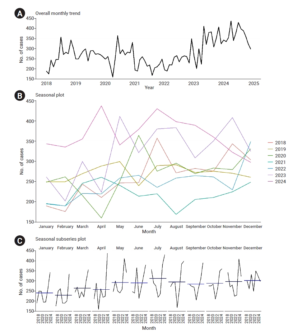
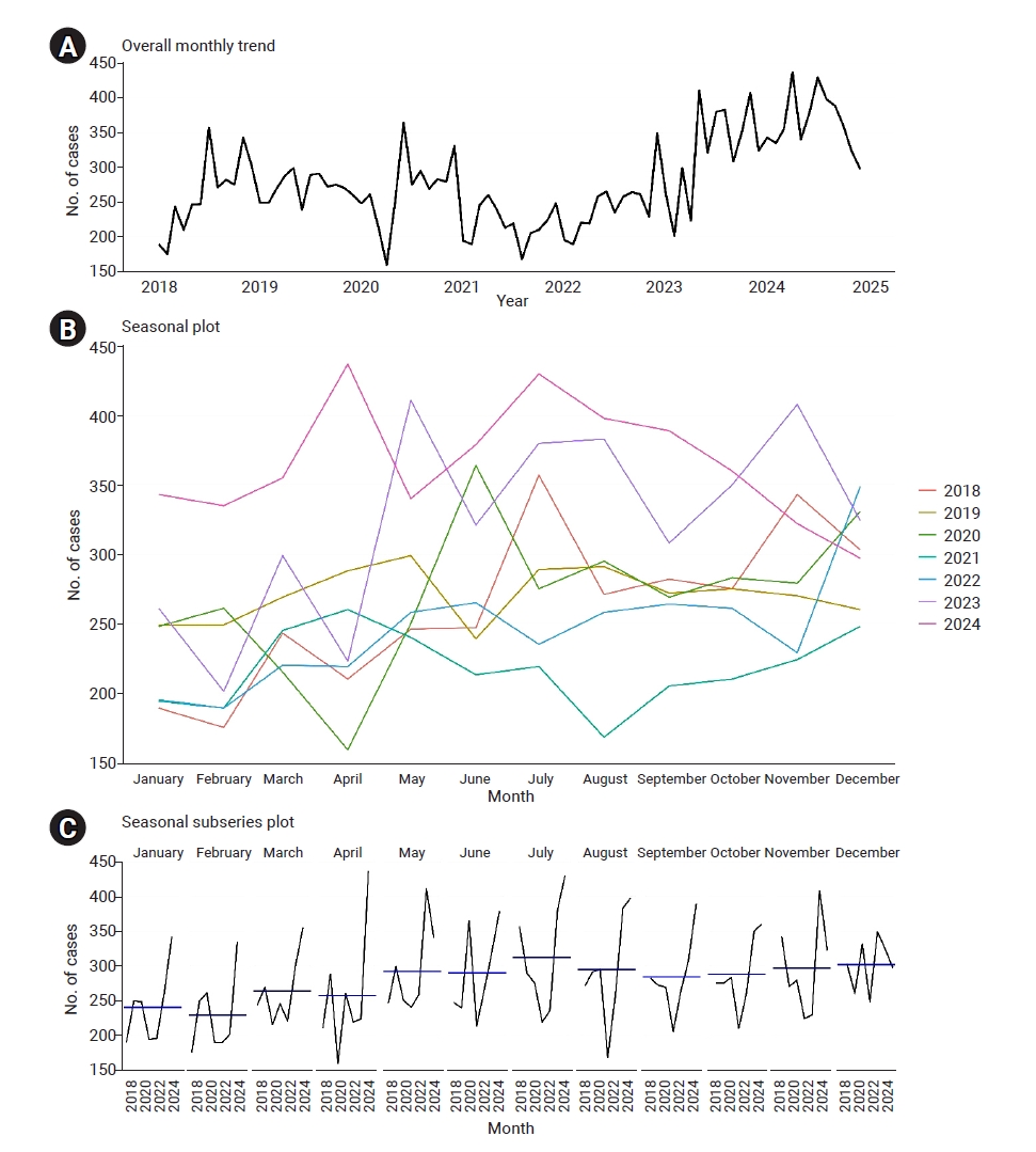
A total of 24,028 laboratory-confirmed NTS cases were included in the analysis. Overall case counts fluctuated from 2018 to 2022, increased markedly in 2023, and peaked in 2024, with annual totals of 2,942, 3,388, 3,359, 2,670, 2,995, 3,826, and 4,848 cases from 2018 through 2024, respectively (
Figure 1A). Monthly laboratory-confirmed NTS cases showed temporal variability, with evidence of both trend and seasonality (
Figure 1). The seasonal plot showed recurring intra-annual variation: in several years, case counts were higher during the mid- to late-year months, although the timing and magnitude of peaks varied (
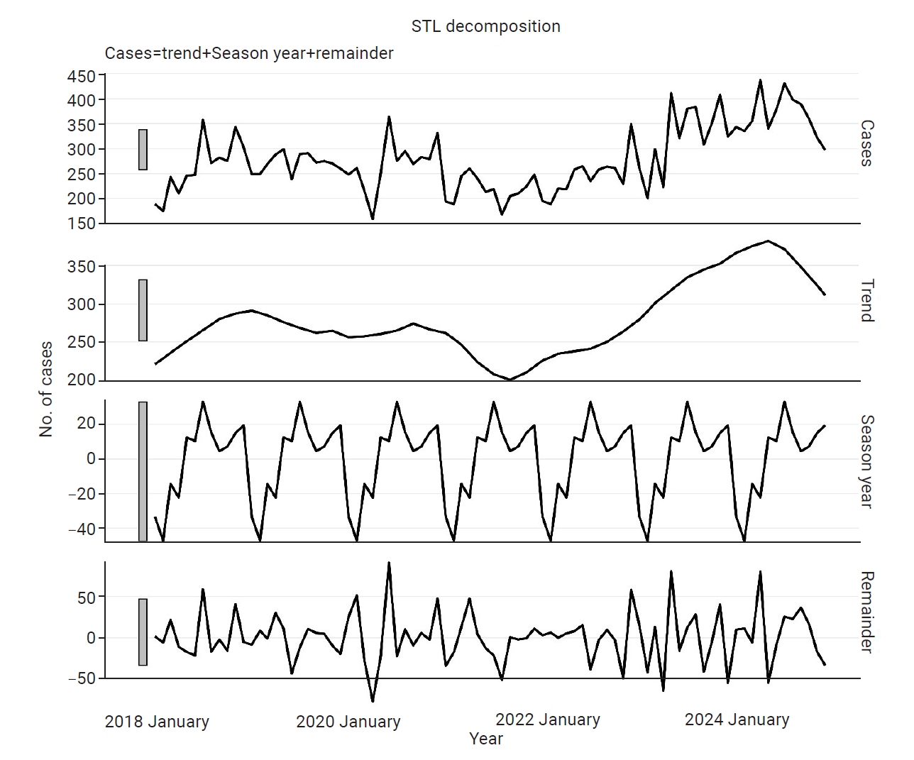
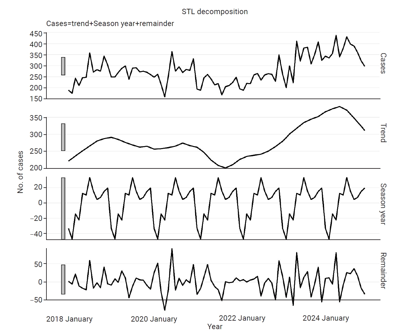
Figure 1B). The seasonal subseries plot further showed month-specific patterns, with April, July, and November having comparatively higher average case counts and greater variability in later years. These patterns were supported by STL decomposition, which identified a strong trend component (trend strength=0.69) and a moderate recurring seasonal component (seasonal strength=0.32), consistent with interannual variation in the timing and magnitude of seasonal peaks. Monthly case counts fluctuated more widely in later years, particularly from 2023 onward (
Figure 2). Unit-root diagnostics showed that the original series was nonstationary (ADF,
p=0.65; KPSS,
p<0.01), whereas stationarity was achieved after first-order differencing (d=1; ADF,
p<0.01; KPSS,
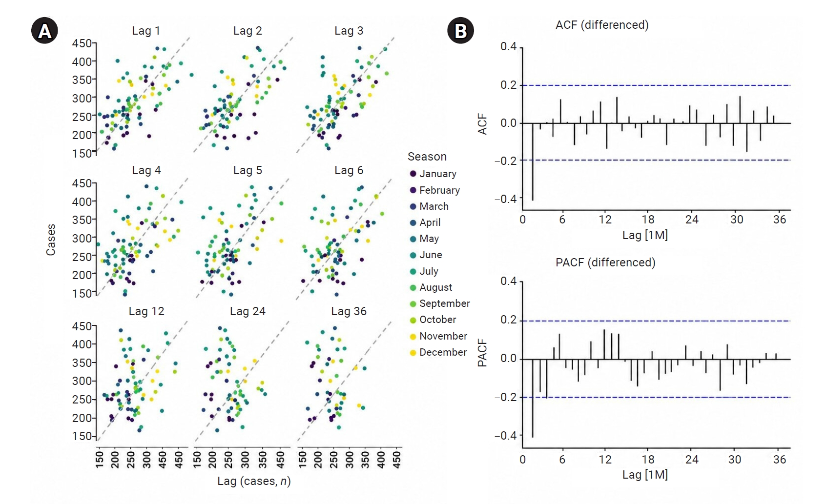
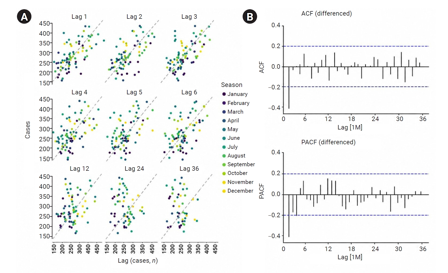
p>0.10). Consistent with the decomposition results, seasonal differencing was not required (d=0). Lag plots showed substantial short-term dependence at lags of 1–3 months, followed by rapid decay, consistent with a short-memory process (
Figure 3). In contrast, the lag-12, lag-24, and lag-36 plots did not show strong linear year-to-year dependence. The ACF of the first-order differenced series showed a significant spike at lag 1 followed by rapid decay, consistent with a first-order MA process (MA=1). The PACF showed a significant negative spike at lag 1 followed by gradual damping, with no notable spikes at seasonal lags, suggesting no clear nonseasonal or seasonal AR components (AR=0). Together, these diagnostics supported the specification of an ARIMA(0,1,1) model, which was also identified as optimal by automated model selection based on information criteria.
The in-sample fit of the candidate ARIMA and ARIMA–Fourier models is presented in
Table 1. Among the seasonal and nonseasonal specifications, ARIMA(0,1,1) had the lowest AICc (753.42), and model fit improved after Fourier terms were incorporated. Although higher-order Fourier models achieved slightly lower AICc values, they produced higher forecast errors, suggesting overfitting (
Tables 1,
2). The more parsimonious ARIMA(0,1,1)–Fourier (
K=1) model was therefore selected because it had the lowest forecast error and outperformed all benchmark and ETS models (
Table 2). Residual diagnostics showed no substantial evidence of heteroscedasticity or residual autocorrelation (Ljung-Box test,
p=0.696). The normal Q–Q plot indicated that residuals were approximately normally distributed in the central range, although tail deviations were observed because of a small number of extreme observations. This pattern supported the use of the model for prediction-interval estimation. All forecast means and corresponding 95% prediction intervals remained above zero.
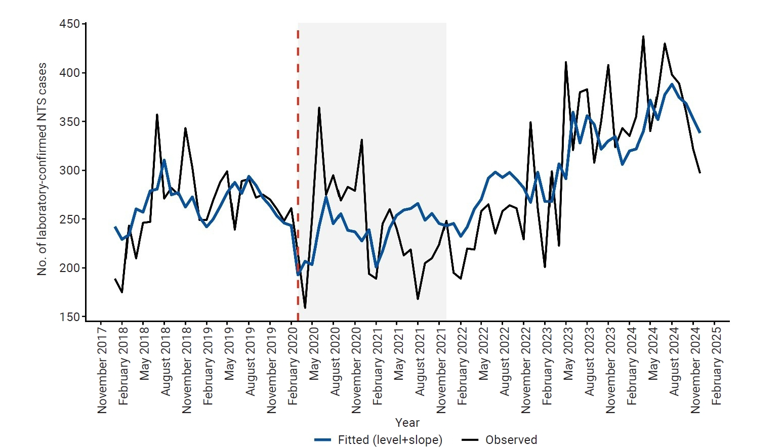
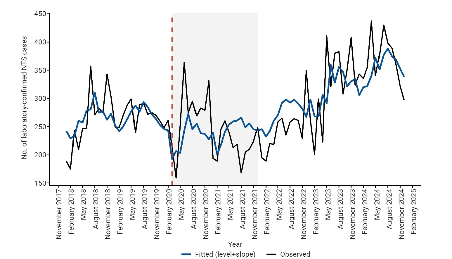
Subsequent ITS analysis showed a significant immediate reduction in NTS cases at the beginning of the COVID-19 pandemic (β=−62.24 cases; 95% confidence interval [CI], −98.96 to −25.52;
p=0.001), followed by a significant positive post-intervention slope (β=2.71 cases/month; 95% CI, 1.83–3.59;
p<0.001), indicating an increasing trend in reported cases after March 2020 (
Figure 4). Among the candidate ITS specifications, the segmented level-and-slope model provided the best fit, with a lower AICc than the level-change and temporary pulse models (894.7 vs. 919.4 and 912.7, respectively). The MA(1) parameter remained significant (
p=0.006), suggesting persistent short-term stochastic dependence.
Exploratory Hybrid ARIMA–LSTM Analysis
The ARIMA–LSTM models showed modest improvements in out-of-sample forecast accuracy compared with the standalone ARIMA–Fourier models (
Table 2). Across configurations, RMSE decreased from 43 cases to approximately 39–40 cases, corresponding to a 7%–8% improvement. Similar reductions were observed for MAE and MAPE. Among the evaluated models, the hybrid B Fourier (
K=1)+LSTM model with 8 units, 200 epochs, and a batch size of 4 achieved the best forecast performance and was therefore selected as the final specification for surveillance evaluation. Month-specific error analysis of this model showed systematic underestimation during several higher-case months in 2024, with the largest forecast error observed in April (ARIMA–Fourier error, −106.48 cases; hybrid error, −98.19 cases). Although both models underpredicted the April surge, the hybrid model reduced the magnitude of forecast error in most months (
Table S1). Across multiple rolling-origin validation periods (
Table 3), the ARIMA–Fourier and hybrid models performed similarly during 2021–2023, with only marginal differences in RMSE. In the 2024 validation period, which was characterized by higher-case counts and greater variability, the hybrid model showed a larger improvement, reducing RMSE by 3.57 cases (8.3%) relative to the ARIMA–Fourier model.
Model-Based Anomaly Detection
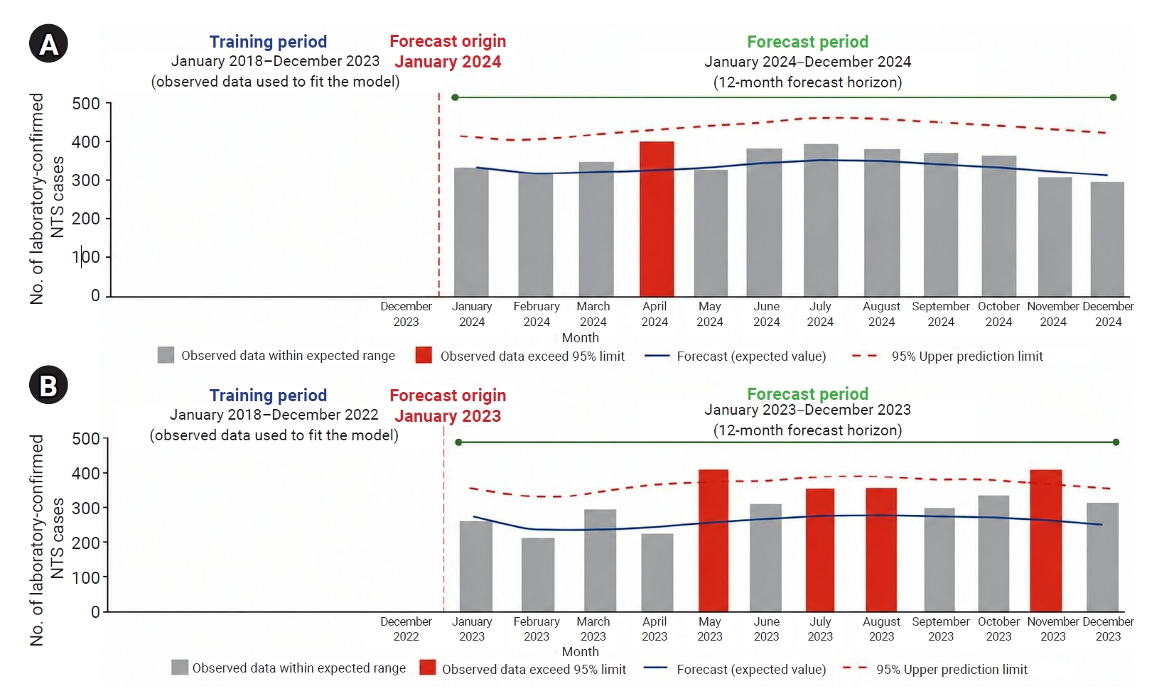
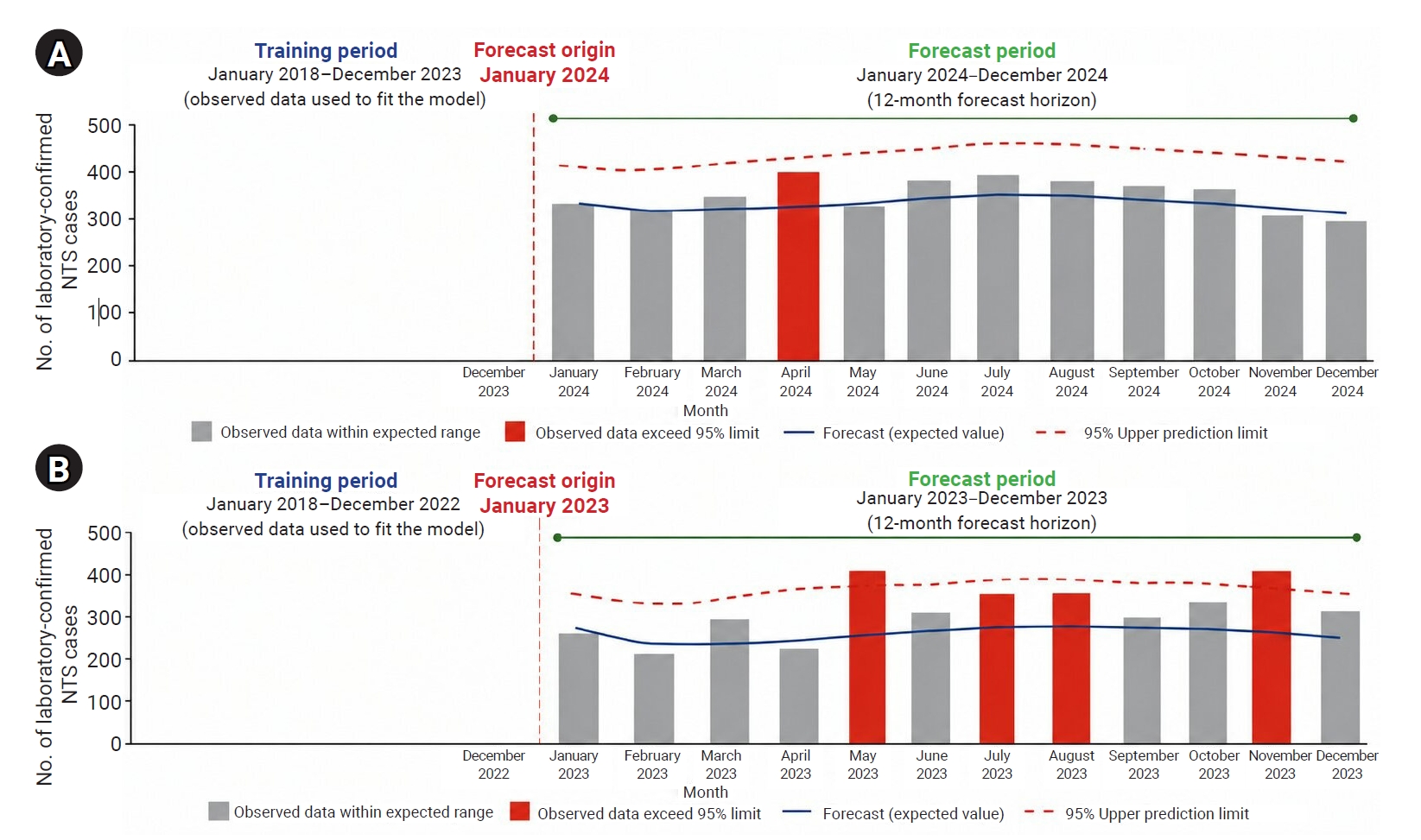
Prediction-interval-based assessment identified observations that exceeded the upper 95% prediction limit of the modeled baseline (
Figure 5). Across the national-level holdout evaluations for 2023 and 2024, 24 monthly observations were evaluated, of which 5 exceeded the upper 95% prediction limit. Under correct model specification, approximately 1.2 exceedances would be expected by chance alone. In 2024, 1 month, April, was flagged; this coincided with 3 large-scale outbreak events reported within the same region. In 2023, significant deviations were observed in May, July, August, and November. In May, increased suspected NTS outbreaks associated with multiple social-gathering events were reported in the Central region. In July and August, multiple outbreaks in the East Coast region were linked to specific serovars,
Salmonella Corvallis and
Salmonella Livingstone. In November, multiple outbreaks reported separately in 3 states and associated with
Salmonella Paratyphi B var. L(+) tartrate were subsequently linked to a common source after DNA fingerprinting initiated by NPHL showed 100% genetic similarity.
Regional Heterogeneity Assessment
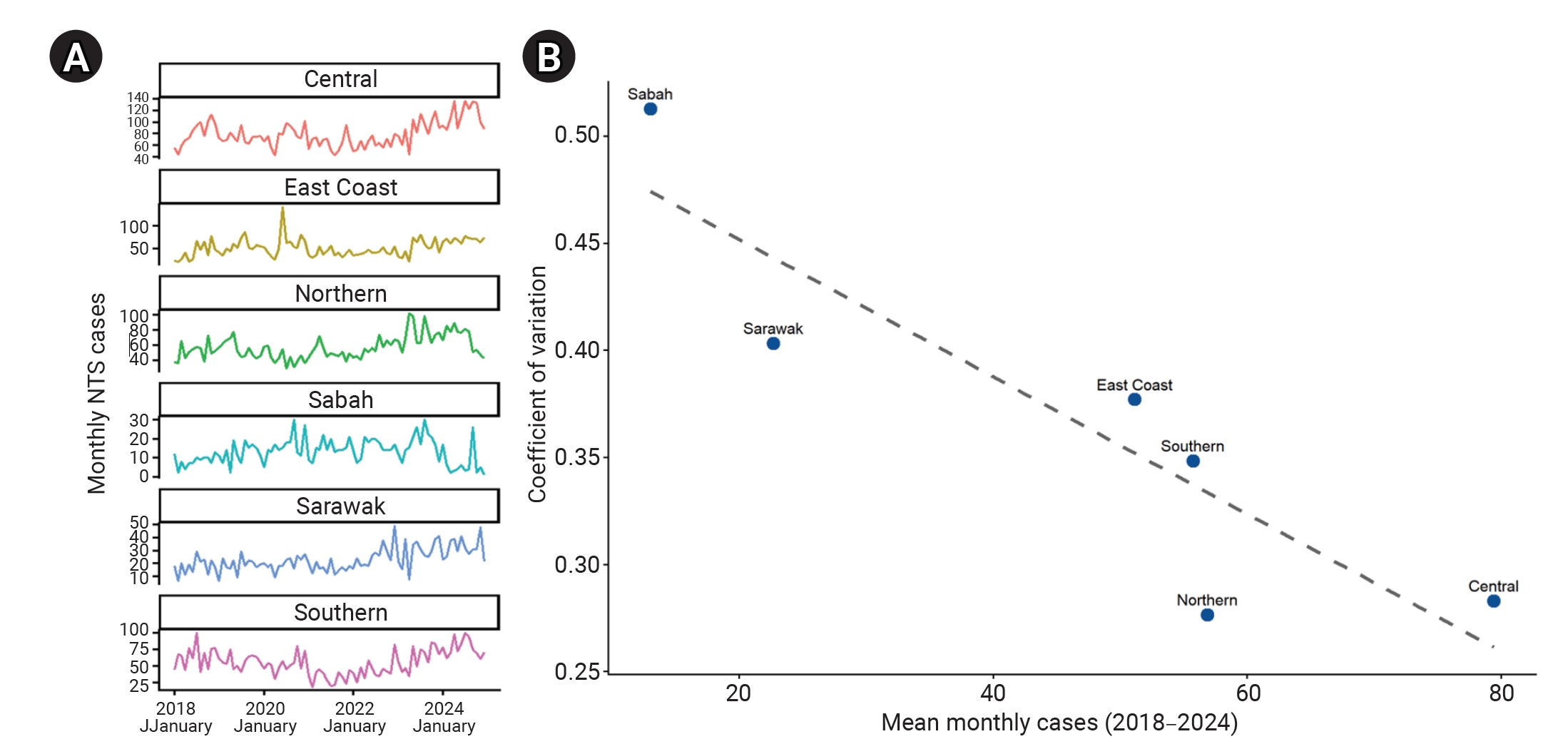
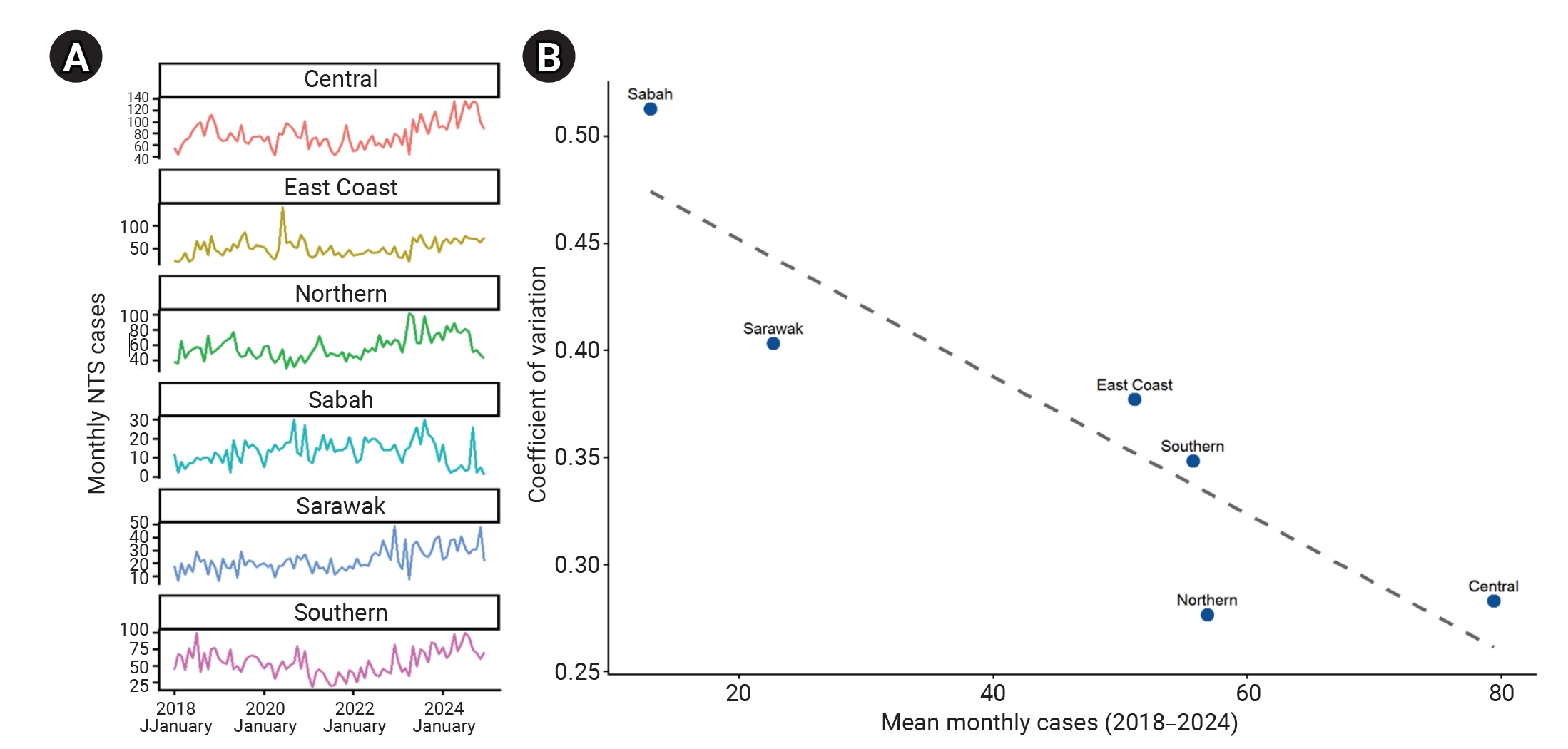
Regional heterogeneity was observed in both case magnitude and temporal structure. Regions with higher mean monthly case counts, such as the Central and Northern regions, showed relatively stable patterns, whereas regions with lower mean monthly case counts showed greater relative variability. This pattern was consistent with a strong inverse correlation between mean monthly cases and the coefficient of variation (Spearman’s ρ=−0.943,
p=0.017) (
Figure 6). Regional decomposition showed generally similar temporal patterns across Malaysia, although the relative contributions of trend and seasonality varied. Sabah had the strongest seasonal component, whereas the East Coast had the weakest trend strength; the remaining regions showed comparable seasonal and trend strengths (
Table 4). Seasonal timing was relatively stable, with consistent peak months across most regions, although peak timing in Sarawak varied between July and December in later years. Applying ARIMA-based models to regional data further showed variation in optimal model structure. When the national ARIMA(0,1,1)–Fourier (
K=1) model was applied to regional series, forecast performance varied across regions (
Table 5). Scale-independent forecast accuracy, measured using mean absolute scaled error (MASE), also differed regionally, with the best performance in the Southern region (MASE=0.73) and the poorest performance in Sabah (MASE=2.30). Residual autocorrelation was highest in the Northern region (ACF1=0.505), indicating that the national ARIMA–Fourier model did not fully capture regional temporal structure (
Table 5).
Discussion
The recurring but variable seasonal pattern of NTS cases observed in this study may reflect the epidemiology of foodborne transmission in tropical settings. Although climatic and behavioral factors were not explicitly examined, the observed seasonal peaks were consistent with known environmental and behavioral patterns in Malaysia. Previous studies have linked NTS transmission to communal dining, festive gatherings, food consumption patterns, agricultural contamination, and environmental conditions that facilitate bacterial proliferation, including heavy rainfall and warmer temperatures [
16–
18]. In Malaysia, the Northeast Monsoon (November–March) is characterized by heavy rainfall and flooding; the inter-monsoon phase (October–November) is marked by intense rainfall and thunderstorms; and the Southwest Monsoon is associated with higher ambient temperatures and heatwaves (February–May) [
19]. Long school breaks during the mid-year and year-end periods may also increase population movement and exposure risk because they often involve large gatherings and intensified food preparation [
20]. The observed monthly variation is broadly consistent with global evidence showing recurring seasonal peaks across countries, although the timing and magnitude of these peaks vary by setting [
21–
23]. The ARIMA–Fourier model provided the best performance among the statistical forecasting models. Although its improvement in forecast accuracy was modest, the Fourier term represented the expected seasonal baseline needed for anomaly detection. The additive seasonal structure adequately captured the overall temporal pattern in this study; however, the increased variability in later years and the underestimation of several higher-case months in 2024 suggest that seasonality alone does not fully explain temporal variation. Changes in trend and seasonal amplitude may also contribute to disease dynamics. Future work should evaluate multiplicative seasonal models or log-transformed time series to determine whether these approaches improve forecasting performance under changing epidemiological conditions. Because this analysis used laboratory-confirmed surveillance data, temporal changes, particularly during the COVID-19 pandemic, may reflect changes in healthcare utilization and case ascertainment as well as changes in disease occurrence. The marked decline during 2020–2021 and the subsequent increase from 2022 onward should therefore be interpreted in the context of the COVID-19 pandemic, when reduced healthcare-seeking behavior, limited access to health services, and diversion of public health and laboratory resources may have affected case ascertainment. Improved healthcare-seeking behavior reported in the 2023 National Health and Morbidity Survey [
24] may also have contributed to the post-pandemic increase in laboratory-confirmed cases.
A key feature of NTS epidemiology is the occurrence of sudden, localized point-source outbreaks, which may arise from contaminated food sources, institutional catering events, or breaches in food safety procedures and can produce sharp increases above expected seasonal baselines [
25,
26]. Although these deviations cannot be fully predicted from historical temporal patterns alone, embedding forecasting models within a prediction-interval framework can help distinguish expected seasonal variation from statistically unusual events. The ARIMA–LSTM approach provided modest improvements in forecasting accuracy, suggesting that adding a nonlinear residual component to a predominantly linear seasonal framework may improve the stability and precision of short-term infectious disease forecasting, consistent with previous studies [
4,
27]. Further examination showed that forecast errors were not uniformly distributed, with larger errors occurring during higher-case periods. Month-level analysis and year-specific validation showed reduced underestimation during peak periods, consistent with short-lived nonlinear dynamics that may emerge when transmission increases. This issue is relevant to surveillance because underestimation during high-case periods may delay recognition of unusual events. However, the added complexity of the hybrid method should be considered carefully. The exploratory ARIMA–LSTM analysis should be interpreted with caution because the limited number of training sequences may increase sensitivity to data partitioning and random initialization. These findings should therefore be considered preliminary and require validation using longer surveillance time series. Accordingly, LSTM use in this study should be interpreted as exploratory, with potential benefits under specific conditions, rather than as evidence that LSTM is generally superior to conventional statistical modeling. For diseases such as NTS, which are characterized by regular seasonal transmission punctuated by episodic outbreaks and interannual variability, this approach may provide a context-sensitive way to improve surveillance sensitivity without increasing false alerts. The modest improvement observed with the hybrid model should also be interpreted in the context of the limited time series. Future evaluation using longer surveillance records may provide a more robust assessment of whether hybrid machine-learning approaches offer meaningful advantages over conventional statistical models.
This exploratory analysis provides a retrospective proof of concept showing that forecast-based anomaly detection can distinguish observed case counts from an expected modeled baseline. Such signals may help identify unusual increases in cases that warrant further epidemiological investigation, particularly to determine whether cases share similar sources or exposure pathways. However, because exceedances of the 95% prediction interval may occur by chance under correct model specification, flagged observations should be interpreted as surveillance signals rather than confirmed outbreaks and should undergo epidemiological verification. We did not formally evaluate outbreak detection performance because complete and reliable outbreak-event data were not available within the laboratory-based surveillance system. Most laboratory-confirmed cases are sporadic, whereas most outbreaks are identified through epidemiological investigations without corresponding laboratory confirmation. Nevertheless, integrating model-based anomaly detection into existing national laboratory surveillance systems may complement routine surveillance by providing retrospective, data-driven signals of unusual transmission patterns that warrant further investigation. Prospective implementation using sequential real-time forecasts and predefined alert thresholds would be required to determine operational performance, including timeliness, sensitivity, specificity, and false-alert rates.
Substantial regional heterogeneity in case magnitude, proportional variability, structural decomposition, and AR behavior was also observed across Malaysia. Regions with lower case magnitudes showed greater proportional instability, consistent with increased stochastic fluctuation in smaller population time series. National aggregation may stabilize temporal signals and improve detection of widespread or multiregional outbreaks, whereas regional series may show greater proportional volatility and distinct AR structures. This volatility reduces forecast stability and limits the reliability of more complex regional-level modeling, with direct implications for surveillance strategy. These findings suggest that national models may be useful for monitoring broad temporal trends and detecting widespread events, especially those involving cross-border exposure or food distribution networks. In contrast, simplified or locally tailored models may be needed to identify localized events or anomalies that do not immediately affect national counts. A tiered surveillance framework, in which national models serve as primary early-warning tools and are complemented by region-specific monitoring for local outbreak detection, may provide a practical balance between operational robustness and early-warning sensitivity. The operational effectiveness of this framework was not evaluated in the present study and should be assessed in prospective surveillance settings.
The ITS analysis identified a marked disruption in reported NTS cases, consistent with global observations during the COVID-19 pandemic. Previous studies have reported declines in NTS infection during the pandemic, attributed to changes in food exposure patterns, travel restrictions, and reduced social mixing, as well as reduced surveillance sensitivity due to reprioritization of laboratory resources for severe acute respiratory syndrome coronavirus 2 testing and reduced healthcare utilization [
28–
30]. Despite the initial decline, the present analysis showed a significant positive post-intervention trend, suggesting a gradual increase in reported cases after the March 2020 interruption. Changes in home food preparation and informal food enterprises may have introduced competing food safety risks, with increased reporting of NTS outbreaks involving privately owned poultry and a shift in exposure settings from schools to restaurants [
29,
30]. Although the segmented ITS model estimated a sustained post-intervention trend, visual inspection of the observed and fitted time series suggested that the marked decline during the early pandemic was transient: reported NTS cases gradually returned toward pre-pandemic levels, and the characteristic seasonal pattern had re-emerged by 2022. This interpretation was further supported by the poorer fit of the temporary pulse model relative to the segmented model, indicating that the interruption was better represented by an immediate decline followed by gradual recovery than by a sustained downward shift. These findings indicate that the pandemic-related interruption can be accommodated through intervention modeling, supporting retention of the full historical dataset for subsequent forecasting rather than partitioning the series into separate pre- and post-pandemic periods.
This study focused on characterizing baseline temporal dynamics for surveillance; however, predicting sudden outbreak-level increases from historical data alone remains challenging. Incorporating environmental, behavioral, and population-related factors into predictive models may further improve performance, but this was beyond the scope of the present analysis. Finer temporal resolution may improve detection of rapid changes and increase the number of data points available for modeling; however, in routine laboratory surveillance, variability in testing, specimen transport, and the sporadic nature of NTS infection may produce inconsistent weekly data. Another limitation is reporting delay within the laboratory-based surveillance process, because NTS isolates are first cultured at healthcare facilities and then transported to reference laboratories. Cases occurring near the end of a reporting period may therefore be recorded in the subsequent month, affecting the temporal precision of forecasting and alert timing. To improve the temporal alignment of monthly or weekly surveillance models, laboratory information systems should prioritize recording and analyzing specimen collection dates rather than dates of receipt at the reference laboratory.
Nevertheless, this study used 7 years of nationwide laboratory-confirmed surveillance data, enabling a detailed assessment of seasonal dynamics and temporal patterns. Integrating ITS analysis with ARIMA–Fourier and hybrid ARIMA–LSTM modeling provided a framework that linked forecast optimization with structural stability assessment. Together, these findings support the combined use of predictive modeling, structural assessment, and routine monitoring to develop model-based approaches for NTS surveillance.
Article information
Ethics Approval
This study was conducted in accordance with the Declaration of Helsinki and the Malaysian Good Clinical Practice Guideline. Ethical approval was provided by the Human Research and Ethics Committee, Universiti Sains Malaysia (JEPeM; USM/JEPeM/22110718). The study was registered with the National Medical Research Register (NMRR ID-22-02749-XAA), and ethical approval was also obtained from the National Institute of Health’s MREC, in accordance with current guidelines. The requirement for informed consent was waived because of the retrospective nature of the study.
Conflicts of Interest
The authors have no conflicts of interest to declare.
Funding
This study was supported by the School of Medical Sciences, Universiti Sains Malaysia (Medical Research Grant 2025 Project No. R501-LRGPP001-0000002020-0000). The funder had no role in the study design; data collection, analysis, or interpretation; or manuscript preparation.
Availability of Data
The datasets generated and/or analyzed during the current study are not publicly available because of institutional data governance policies but may be made available upon reasonable request, subject to approval by the Ministry of Health Malaysia.
Authors’ Contributions
Conceptualization: HMH, KIM, SMH, NMHMF; Data curation: HMH, NM, NS, AA, RI, RH; Formal analysis: HMH, KIM, SMH; Methodology: HMH, KIM, SMH, NMHMF; Project administration: HMH, KIM, RI; Supervision: KIM, SMH, JWJN; Visualization: HMH; Writing–original draft: HMH; Writing–review & editing: all authors. All authors read and approved the final manuscript.
Acknowledgements
This study was supported by the School of Medical Sciences, Universiti Sains Malaysia. The authors gratefully acknowledge this support. The authors thank the Director General of Health Malaysia for granting permission to conduct this research and publish this article.
An AI language model (ChatGPT, OpenAI, GPT-5.3) was used solely to improve readability and clarity, including grammar and style. It was not used for data analysis or for generating scientific content. All outputs were reviewed and approved by the authors, who take full responsibility for the manuscript. No AI-generated material is cited as a primary source.


 , Kamarul Imran Musa1